Previous: Chapter 5. Maxwell’s Demon and Information
In previous chapters, it was shown how the Gibbs statistical entropy was used to justify the subjectivity of entropy and its relationship to information entropy. As a result, a number of physicists who advocate the objectivity of entropy have chosen to abandon the use of the Gibbs method for foundation of statistical mechanics. Their position can be summarized by the slogan ‘Back to Boltzmann’. They have proposed to modify the Boltzmann entropy to the general case by means of a transition to Γ-space.
The modified Boltzmann entropy is related to the treatment of non-equilibrium states in statistical mechanics. I examine the use of the modified Boltzmann entropy with an example of the candle combustion in an isolated system. This allow us to compare non-equilibrium states in statistical mechanics and continuum mechanics, as well as discuss the existence of new non-equilibrium states that do not have counterparts in continuum mechanics.
The ‘Back to Boltzmann’ path exclude time in the explicit form. At the same time, non-equilibrium statistical mechanics is used to derive kinetic equations. In practice, different characteristic relaxation times are employed and a hierarchy of approximations is made. Thus, problems to find the arrow of time do not hinder the discovery of useful solutions. Moreover, in practice, priorities are reversed, the first task is to derive kinetic equations, and the entropy change is pushed to the background.
- Back to Boltzmann!
- Macrostate entropy
- Non-equilibrium macrostates and microstates
- Entropy of non-equilibrium states and kinetics
- Non-equilibrium statistical mechanics in practice
Back to Boltzmann!
A number of physicists would like to preserve the objectivity of entropy, and therefore they advocate a return to Boltzmann’s method as foundation for the arrow of time; for the Gibbs statistical entropy, a service role only is left. I quote from the conclusion of the paper by theoretical physicists ‘Gibbs and Boltzmann entropy in classical and quantum mechanics‘:
‘The Gibbs entropy is an efficient tool for computing entropy values in thermal equilibrium when applied to the Gibbsian equilibrium ensembles, but the fundamental definition of entropy is the Boltzmann entropy. We have discussed the status of the two notions of entropy and of the corresponding two notions of thermal equilibrium, the “ensemblist” and the “individualist” view. Gibbs’s ensembles are very useful, in particular as they allow the efficient computation of thermodynamic functions, but their role can only be understood in Boltzmann’s individualist framework.’
To a greater extent, this point of view is dramatized in the works of philosophers of physics, who search for an ideal foundation for statistical mechanics. Below there are quotes from the paper ‘Philosophy of Statistical Mechanics‘ (BSM and GSM refer to Boltzmann and Gibbs statistical mechanics, respectively):
‘philosophical discussions in statistical mechanics face an immediate difficulty because unlike other theories, statistical mechanics has not yet found a generally accepted theoretical framework or a canonical formalism.’
‘Finally, there is no way around recognising that BSM is mostly used in foundational debates, but it is GSM that is the practitioner’s workhorse. When physicists have to carry out calculations and solve problems, they usually turn to GSM which offers user-friendly strategies that are absent in BSM. So either BSM has to be extended with practical prescriptions, or it has to be connected to GSM so that it can benefit from its computational methods.’
Let’s consider a picture from the website universe-review.ca – Thermodynamics:
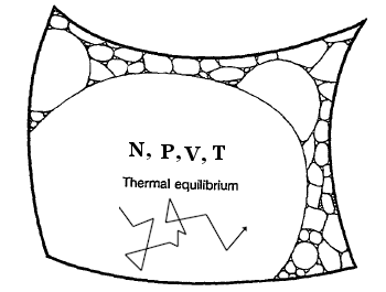
The surface of the phase space with a given energy is shown in the figure. In reality, this surface is of very high dimensionality, but a simple plane is used for simplicity. Each cell represents a macrostate with many microstates, and the area of the cell is proportional to the number of microstates. The largest cell represents an equilibrium state with uniform temperature, while the other cells represent non-equilibrium states. The difference with the Boltzmann equation is the transition from μ-space to Γ-space and the replacement of the number of permutations with the area of the surface in Γ-space. The transition to Γ-space allows us to speak about the universality of such an explanation.
Below there are quotes from Roger Penrose’s book ‘Fashion, Faith, and Fantasy in the New Physics of the Universe‘, which explain the idea shown in the picture in more detail:
‘What, then, is this “measure of entropy”? Roughly speaking, what we do is to count all the different possible submicroscopic states that could form a particular macroscopic state, and the number of these states N is a measure of the entropy of the macroscopic state. The larger N is, the greater the entropy.’
‘This is, indeed, essentially the famous definition of entropy given by the great Austrian physicist Ludwig Boltzmann in 1872.’
‘it is best that we return to the notion of phase space … the phase space P, of some physical system, is a conceptual space, normally of a very large number of dimensions, each of whose points represents a complete description of the submicroscopic state of the (say, classical) physical system being considered.’
‘Now, in order to define the entropy, we need to collect together – into a single region called a coarse-grained region – all those points in P which are considered to have the same values for their macroscopic parameters. In this way, the whole of P will be divided into such coarse-graining regions. … Thus, the phase space P will be divided up into these regions, and we can think of the volume V of such a region as providing a measure of the number different ways that different submicroscopic states can go to make up the particular macroscopic state defined by its coarse-graining region.’
It is important to note that the picture above is not scaled correctly, and the areas of the non-equilibrium states have been exaggerated for clarity. In the equilibrium microcanonical distribution, the statistical weight corresponds to the entire area in the figure, including the non-equilibrium states. This means that the equal a priori probability principle includes all states, both equilibrium and non-equilibrium, and in turn it shows that the area corresponding to the equilibrium macrostate cell is significantly larger than the areas of the non-equilibrium state cells; the latter would be almost invisible on a proper scale.
Macrostate entropy
The macrostate entropy in the new approach is related to the statistical weight of a single cell Wv in the Γ-space:
S = k ln Wv
The statistical weight of the equilibrium state using Wv is almost equal to the statistical weight using the entire area, so the entropy of the equilibrium macrostate is indistinguishable from the entropy in the equilibrium microcanonical ensemble. At the same time, this approach defines the entropies of non-equilibrium states, which can be used now as a foundation for the arrow of time. Penrose gives the final conclusion as follows:
‘In order to see how this helps in our understanding of the 2nd Law, it is important to appreciate how stupendously different in size the various coarse-graining regions are likely to be, at least in the kind of situation that is normally encountered in practice. The logarithm in Boltzmann’s formula, together with the smallness of k in commonplace terms, tends to disguise the vastness of these volume differences, so that it is easy to overlook the fact that tiny entropy differences actually correspond to absolutely enormous differences in coarse-graining volumes. … Since the (vastly) larger volume corresponds to an (albeit usually only slightly) larger entropy, we see, in general rough terms why the expression for the entropy increases unstoppably over time. This is exactly what we would expect according to the second law.’
Proponents of the new approach argue that the connection of microstates with macrostates excludes subjectivity in the entropy of non-equilibrium states. In parallel, the concept of typicality (typical behavior) is introduced and it is considered as a solution to the Loschmidt and Zermelo paradoxes. For example, the figure above shows that the reversal of velocities for the absolute majority of microstates in the equilibrium state leaves the trajectory of the system in this cell. The direction of the trajectory plays a role only for a negligible number of microstates that are at the boundary of the macrostate; in this sense, the trajectories in the equilibrium state represent the typical behavior of the system.
The figure above also allows us to better understand Carnap’s logic related to the entropy of a microstate. A macrostate corresponds to a system under study, and a macrostate has entropy. On the other hand, the macrostate under study belongs to a specific trajectory of the system, which is a sequence of microstates that belong to the solution of the Hamilton equation of motion. Carnap’s principle of physical magnitudes requires that the entropy in both cases be consistent within the experimental errors; this requires the presence of entropy of the system for a specific trajectory of motion.
Non-equilibrium macrostates and microstates
To find the connection between macrostate and microstates, Boltzmann used the discretization of cells by the values of coordinates and momenta in μ-space. However, this is impossible in Γ-space, and this is the main problem with the modified Boltzmann equation for the entropy of non-equilibrium states. The equation expresses an idea, but it remains unclear how it could be possible to implement it.
The general idea is to introduce the properties of a macrostate, and then to enumerate the microstates. For each microstate, macroscopic properties should be evaluated, and this way microstates could be distributed among the macrostates. Of course, this procedure is not feasible in practice, but it is assumed that it is possible in principle. In his book Penrose immediately moves on to the universe and the problem of the so-called past hypothesis, which addresses the origin of the low-entropy state in the Big Bang. I limit myself to a more prosaic example of the candle combustion — whether such an idea is possible even in principle.
Let us start with a non-equilibrium state in continuum mechanics, which is characterized by fields of temperature, pressure, and concentrations. The goal is then to determine the necessary fields from a given microstate to compare it with one of the macrostates in continuum mechanics. I believe that this task is unsolvable. Let us consider this issue with the temperature field as an example. We need to convert the coordinates and impulses of all particles in a given microstate into temperature field. In kinetic theory, there is the relationship between temperature and the average kinetic energy of atoms, but this equation is only valid for systems in equilibrium. A more correct way for temperature in statistical mechanics is associated with the achievement of the Maxwell-Boltzmann distribution and with the identification of thermodynamic temperature with the parameter of the Maxwell-Boltzmann distribution.
Hence, the correct way to find the temperature field for a microstate is to introduce a local Maxwell-Boltzmann distribution and identify the local temperature with the parameter of this distribution; this is analogous to the principle of local equilibrium. It remains unclear how this task can be practically accomplished for a given microstate, since at the microstate level a much richer choice of nonequilibrium states appears compared to those in continuum mechanics.
Relaxation time is needed for the energy to be redistributed among different degrees of freedom, and therefore there are macrostates in which there are Maxwell-Boltzmann distributions with different values of the temperature for different degrees of freedom. In these macrostates, the translational, rotational, and vibrational temperatures differ from each other. Statistical mechanics has demonstrated the possibility of new states that were not even imaginable in continuum mechanics.
Other non-equilibrium macrostates are associated with the case where local equilibrium is not reached for all degrees of freedom — the case of non-equilibrium temperature or absence of temperature. Thus, there are macrostates for which relaxation is needed to establish the local Maxwell-Boltzmann distribution. The concept of entropy in such states is beyond the entropy of classical and non-equilibrium thermodynamics, although from experience it is expected the relaxation processes are rather fast.
The question is as to whether in the generalized Boltzmann method one can unambiguously determine to which macrostate a given microstate belongs. Such a postulate forms a basis for the generalized Boltzmann method, but it remains unclear whether this problem can be solved even in principle.
Entropy of non-equilibrium states and kinetics
In the modified Boltzmann method, the same problem remains as in the original Boltzmann method. It is assumed that the macrostates are ranked according to their entropy value, as in classical thermodynamics, but time is completely absent. However, in many cases, introducing a typical behavior of the system without actual kinetics is not sufficient. Below the example from Chapter 1.6, ‘Entropy of Non-Equilibrium States‘ is employed.
The absence of time is a distinctive feature of classical thermodynamics. It is possible to predict the direction of a spontaneous process, but it is impossible to say how quickly the process occurs. During the development of thermodynamics and continuum mechanics, this served as a distinction between thermodynamics and transport processes in continuum mechanics. The Clausius inequality belonged to classical thermodynamics, while the question of the process time belonged to kinetics and continuum mechanics. Statistical mechanics, on the other hand, contains time and it should provides an explanation for all processes, including the transport equations of continuum mechanics. The absence of time in the modified Boltzmann method limits the scope of applications of statistical mechanics.
Discussing the typical behavior of a system without taking into account the actual kinetics is insufficient. Let us take a candle in air atmosphere in an isolated system. The final global equilibrium state is related to the combustion products, but the combustion does not start on its own. Therefore, a candle in air atmosphere is also an example of a typical behavior. In this case, statistical interpretation of entropy does not explain why the system does not spontaneously move from a state with lower entropy to a state with higher entropy.
On the other hand, explicit inclusion of time is necessary when considering the process of candle combustion. This process continues for a significant amount of time and can also be considered as a typical behavior. Candle combustion is kind of a quasi-stationary process, as new reactants are continuously added to the reaction, but the flame remains in a relatively stable state. To achieve such a state, specific rates must be maintained. It is unclear how the modified Boltzmann equation could be useful in this case.
Non-equilibrium statistical mechanics in practice
Let us return to the Gibbs method in non-equilibrium statistical mechanics. The problem with the Gibbs statistical entropy is with the Liouville theorem, according to which the Gibbs statistical entropy remains constant in an irreversible process in an isolated system. However, these are general equations that cannot be used directly for practical work as they cannot be solved. This is just a short form of extremely long mathematical equations that is only sufficient to prove general mathematical theorems.
The way to practical problems in non-equilibrium statistical mechanics is based on a hierarchy of approximations, similar to what happens in equilibrium statistical mechanics. Since the goal is to deal with kinetic experiments, such as relaxation processes, the priority belongs to kinetics and not to the entropy of non-equilibrium states. As a result, the Liouville theorem does not hinder the use of non-equilibrium statistical mechanics for practical applications.
Let me take the book by Zubarev, Morozov and Röpke ‘Statistical Mechanics of Nonequilibrium Processes‘ as an example. The authors discuss the problem of Gibbs entropy and suggest possible solutions related to the order of averaging. However, the coarse-graining and fine-graining Gibbs entropies are not used during solution of practical problems.
The non-equilibrium states beyond the scope of continuum mechanics are treated by means of different characteristic times; as a result, there are different approaches to the kinetics of processes at different stages. The book deals with simplified description of non-equilibrium systems and three different regimes with different characteristic times are introduced: dynamic, kinetic, and hydrodynamic. First, there is fast relaxation kinetics followed by a transition to a regime close to the Navier-Stokes equations. The entropy in the book is considered only after the kinetic equations have been derived.
For practical problems, it is necessary to find probability distributions that are relevant to the system in question. In the book, the formalism of the non-equilibrium statistical operator is developed. There are also other methods for finding relevant probability distributions, such as the Zwanzig-Mori projection operator method. In general, physicists understand the specifics of the required solutions and there are no particular problems with using the Gibbs method. Because of the approximations employed to find kinetic equations, the entropy of the system increases as expected.
In conclusion, a few general words. Three levels can be distinguished in statistical mechanics:
- The level of general equations that cannot be solved even in principle; at this level, general mathematical theorems are proved. The conceptual problem related to the arrow of time and the time-reversible laws of physics belongs to this level.
- A hierarchy of approximations that allows us to obtain computational equations for practical applications. In equilibrium statistical mechanics, this allows us to estimate the thermodynamic properties of substances, while in non-equilibrium statistical mechanics, it allows us to obtain kinetic equations.
- Comparison with experimental results.
In the third part of the book, we discuss transitions between levels, mostly with examples in classical thermodynamics and equilibrium statistical mechanics. The discussion of non-equilibrium statistical mechanics will be related to the transport processes of continuum mechanics.
Next: Part3. What does physics say?
References
Sheldon Goldstein, Joel L. Lebowitz, Roderich Tumulka, and Nino Zanghì. Gibbs and Boltzmann entropy in classical and quantum mechanics. In Statistical mechanics and scientific explanation: Determinism, indeterminism and laws of nature, pp. 519-581. 2020.
Roman Frigg and Charlotte Werndl, Philosophy of Statistical Mechanics, The Stanford Encyclopedia of Philosophy, 2023.
Roger Penrose, Fashion, Faith, and Fantasy in the New Physics of the Universe, 2016. 3. Fantasy. 3.3. The second law of thermodynamics.
D. N. Zubarev, V. Morozov, G. Röpke, Statistical Mechanics of Nonequilibrium Processes, 1996.
Additional Information
Entropy in Statistical Mechanics: Back to Boltzmann. doi:10.20944/preprints202602.0005.v1
Boltzmann Statistical Entropy. Gibbs Statistical Entropy. Phase Space Mixing. From Gibbs Entropy to Subjective Entropy. Carnap for Objective Entropy. Back to Boltzmann. Macrostate Entropy. Non-Equilibrium Macrostates and Microstates. Kinetics.
Discussion